A Guide to Deliver a Full ML Pipeline

How to release a model across your organization in one morning (and stop spending excessive amounts of time on a model that will never go into production)

What is this Guide about ?

This guide is a walkthrough for delivering a complete Machine Learning Project by using the Provision.io platform in a very short amount of time.

The guide details each step of a Machine Learning project, from data to model usage across the organization, and shows how to accomplish this within the platform.

What’s in this guide ?

Starting point

This guide assumes that :

You want to create a weekly sales forecast
You have a free version of the io platform
Your IT Team (or data team) has historical sales data in a database and given you access ( but if not, csv files are provided below for the sake of this guide )
An objective has been defined by the Line of Business (LoB)

Steps

The steps of our guide are defined in the chart below:

Steps of a Machine Learning Project

Step	Name	Goal	LoB	IT	Datalab	Output	time spent
1	Data acquisition	Access the historical data for training Machine Learning Model	No	Yes	Yes	dataset	5mn
2	Feature engineering	Prepare the dataset	No	No	Yes	Holdout and validation strategy ( fold )	20mn
3	Define the problem	Define a metrics that reflects LoB process	Yes	No	Yes	An agreement	As Much as possible
4	Experiment	Train models	No	No	Yes	~100 Models	25mn
5	Evaluate	Select the fittest model	Yes	No	Yes	A selection of 3 to 4 models that go into production	As Much as possible
6	Deploy	Share the model across the organization	No	No	Yes	Webapp for human, API for machine	5mn
7	Schedule	Schedule predictions	Yes	Yes	Yes	Prediction delivered each Monday a 9:00 am in CRM software	20mn
8	Monitor	Track the model	Yes	No	Yes	Dashboard	As Much as possible
TOTAL							1h15

For each step, the guide explains what to expect and how we accomplish it on the Provision.io platform.

Results

At the end of this guide :

LoB will receive a weekly sales forecast each Monday at 09:00 am
LoB will receive a simulator for testing hypothesis over the model
Applicative team will get an API for calling the model in their own Application
IT Team will get a dashboard to monitor model Quality of Service

You can open a free account to practice the following steps. When your account is ready, create a Project to host the assets

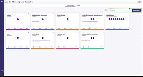
Create a new project

Data acquisition

The first step to any project is getting historical data in order to train our algorithm. As the name implies, Machine Learning is all about reading historical data and letting a computer model learn to predict a target, at least for supervised use cases.

The data should have been loaded into a database by the IT Team and they have generated credentials for you. Once you have created your project, and selected it:

Go to the data section ( sidebar on the left )
Create a new connector and provide the credentials
Create a new datasource from the db and table of past sales
Import it as a dataset

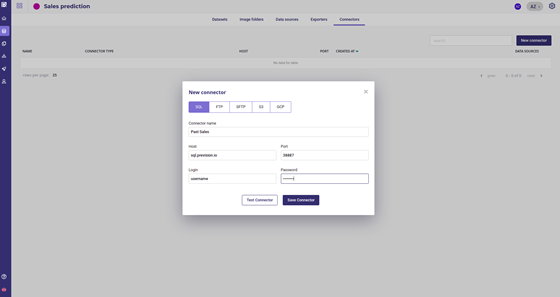
Create a new connector

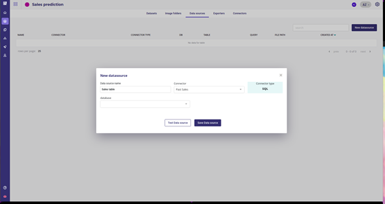
Create a new datasource

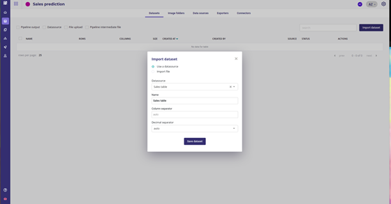
Import dataset

If available, you could import recent sales as a holdout dataset in order to validate and check the stability of your model.

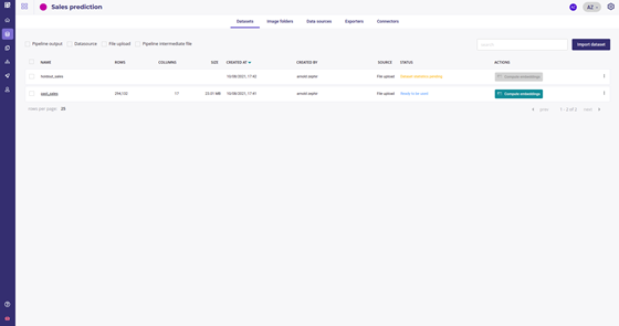
You have two datasets.

Data acquisition is done, you can now start to model.

Status

Task	Status	Output	Time spent
Data acquisition	Done	one trainset, one holdout	5mn

If you don’t have database credentials, you can use the following files. Just import the file instead of using a datasource when importing the dataset.

Feature engineering

Feature engineering is the addition or transformation of one or more features to create new features from the original dataset. In the Provision Platform, and most of the modern tools, feature engineering is done with components and pipelines, yet in most cases you don’t need to add features as the AutoML engine makes all of the standard feature engineering by itself.

Here we are going to add a fold column on the date features in order to properly evaluate our model stability. A specific component has been developed by the data science team starting from the Provision Boilerplate and pushed on a private repo.

The component may now be integrated into the component library of the project.

Go to the pipelines section of your project and under the Pipeline Components tab, click New pipeline Component

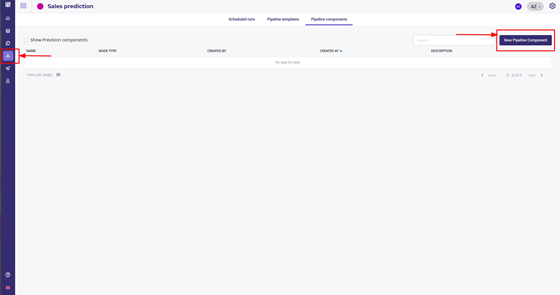
Create a new component

And select your repo and branch.

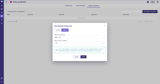
Import component from your repo

Once the component is built, its status will be ok and we can use it in a pipeline. Create a new pipeline template with three nodes:

An import dataset, to read the trainset
The newly created component ( “build fold” )
A save dataset node to save the feature engineered dataset into you Data

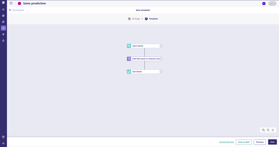
A simple feature engineering pipeline

Then create a new schedule run that you are going to execute manually once on your trainset.

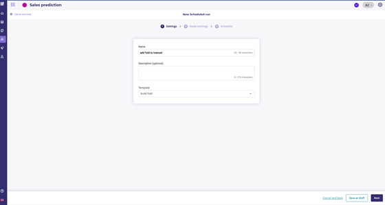
Create a new scheduled run

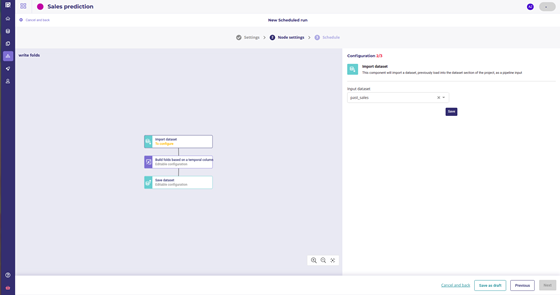
Set your trainset as the input dataset

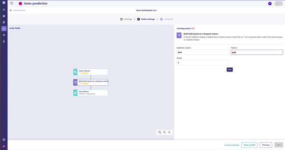
configure your fold component parameters

Once you have done the configuration, select “Manual” as the trigger and run your Schedule run. In a few seconds, a new dataset should be available in your data section as a pipeline output with a new fold column.

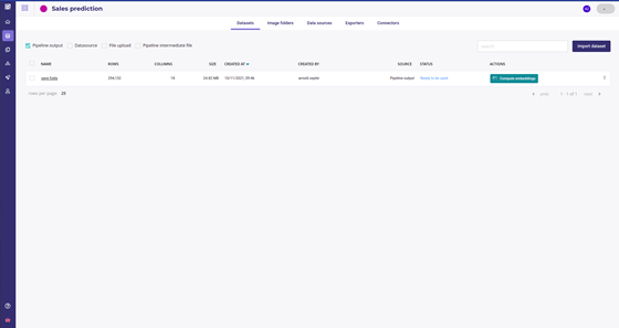
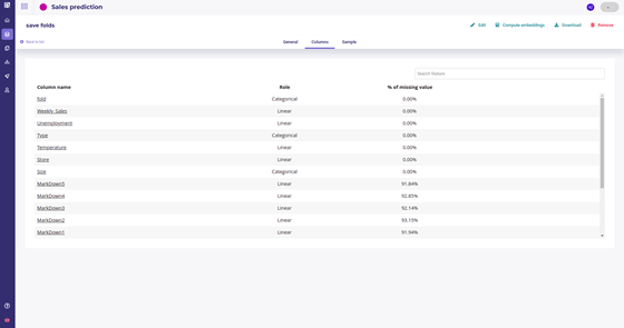
Pipeline output dataset

You now have a dataset with features for a training model and a holdout to validate your models.

Status

Task	Status	Output	Time spent
Data acquisition	Done	one trainset, one holdout	5mn
Feature engineering	Done	one engineered dataset with features, one holdout	20mn

For the sake of this guide, we built a very basic feature engineering pipeline, but you can add as many transformations as you want and build a very complex pipeline.

Here we only have one component that adds a fold column, which is the year modulo 4. You can make the feature engineering on your local machine with the following code. Yet, if you want to build your own component you can follow this guide or some others.

def addfold(df: pd.DataFrame, dtcol: str="dt", foldon:str="year", nfolds:int=3) -> pd.DataFrame:
    if nfolds <=0 :
       nfolds=3
 
    df[dtcol] = pd.to_datetime(df[dtcol])
    df["fold"] = df[dtcol].dt.month % nfolds
 
    if foldon=="year" :
       df["fold"] = df[dtcol].dt.year % nfolds
   if foldon=="day" :
      df["fold"] = df[dtcol].dt.day % nfolds
   if foldon=="hour" :
      df["fold"] = df[dtcol].dt.hour % nfolds
   return df

Define the problem

This is the most important part and the one that should be allocated the most time.

In this step, you’re going to define with the Line of Business how to qualify the project as a success and you, as a data scientist, are going to translate this as data science metrics.

Regression metrics

Choosing the best metrics is out of the scope of this document but you must spend time with your business teams and ask these kinds of questions:

Imagine that I have the perfect model, does it make me gain something?
How much money do I lose if I forecast 110 sales instead of 100?
How much money do I lose if I forecast 90 sales instead of 100?
Are all the predicted products equal?
Should I forecast the total number of items sold, the total amount of sales (in € or $) ), the total weight of my items or the total volume?
How much time before should I forecast?

As a data scientist, by using an AutoML platform, your role is not to code in python or create dockerfiles, but to transcribe business problems to Machine Learning parameters.

In the Provision Platform, you can build what is called an Experiment to help refine your objectives.

Status

Task	Status	Output	Time spent
Data acquisition	Done	one trainset, one holdout	5mn
Feature engineering	Done	one engineered dataset with features, one holdout	20mn
Define the problem	Done	a metric to validate the models	1 week

Experiment

An experiment is a set of Model Building with slightly different parameters across each version and a common Target as well. On each experiment, many models will be automatically built, evaluated in cross-validation and on the holdout dataset if you provide some.

In our case, the models will be trained on our engineered dataset with a fold column and evaluated on a holdout provided by the IT Team.

It is very important to have a good validation strategy to guarantee that the model built in the experiment phase will stay stable on production. Here we choose to :

build a fold column on the modulo of the year number so that we stay confident that the model learned some trends that stay stable over the year
Validate on a holdout with sales from a year that was not in the trainset

Hence, if the holdout score is near to the cross validation score, we know that our model is going to hold up when launched in production and shared across the company.

For creating a new experiment, go to the Experiments section of your project and click New Experiment. You could choose to import some external models if you have some, but here we are using the AutoML Provision Engine. As we want to forecast sales, choose “Tabular” and “Regression”. Give a name to your experiment and click “Create experiment”.

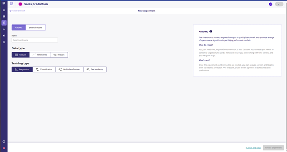
Setting the experiment up

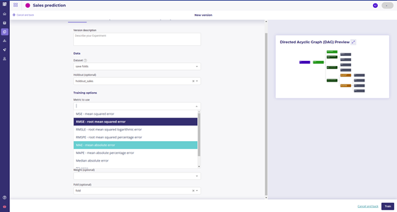
When you create a new experiment, there is no version of the experiment existing so you will be prompted to create a new version. The next screen is where you set up all of your experiment parameters:

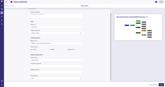
Experiment parameters

The train dataset : use the output of the Schedule run from the step 2 with engineered features
The holdout dataset : use a dataset with the same target as the trainset but with data that are not in the trainset
The metric : use the best metrics that solve the business objectives defined in step 3. You can change it on each version of your experiment so run as many versions as you need if you are not sure
set your target ( here we choose “Weekly Sales” )
and set the fold column up, using the column built during the feature engineering phase.

Note that you may go to the models and feature engineering tabs to change some automl configuration but in most cases the default configuration is fine.

Once done, click on train to launch the training. The platform will immediately start to build and select models with the best hyper parameters. The models will stack in the “models” tabs of your experiment:

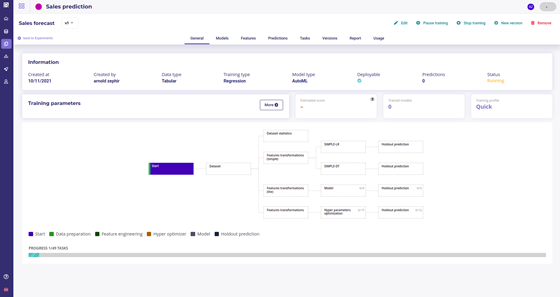
The experiment dashboard

Note that you can launch another version of your experiment as soon as you want, for testing other metrics for example, by using the new version button in the top right corner.

If you have several versions, the experiment dashboard will always display the last version, but you can change to another version with the version dropdown menu or the versions list tabs.

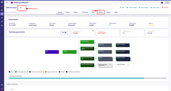
The experiment dashboard

You can launch as many versions as you want and they will run in parallel. You can now grab a coffee and wait till models are built! Depending on the size of your dataset and the plan you subscribed to, expect to wait from 10 minutes to 2 hours before having enough models to evaluate your experiment. In our case, we got our model in approximately 20 minutes.

Status

Task	Status	Output	Time spent
Data acquisition	Done	one trainset, one holdout	5mn
Feature engineering	Done	one engineered dataset with features, one holdout	20mn
Define the problem	Done	a metric to validate the models	1 week
Experiment	Done	~100 models	~20mn

Evaluate

After a few minutes, you should have between 15 and 40 models for each version, depending on which option you choose.

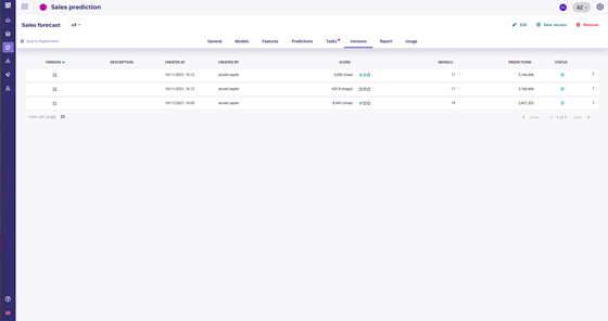
List of experiment versions

This step is all about evaluating all the models produced and selecting 2 to 4 models to deploy for testing in real conditions.

First, have a quick look at the list of versions below ( tab versions of your experiment ). There is a small 3-star evaluation that gives you information about each version’s quality. In this instance, Version 3, which has been trained on Mean Absolute Error, looks the most promising. Click on the specific version to enter the version dashboard for the deepest analysis.

On the Version dashboard, you have several indicators, but the most important is the models comparator :

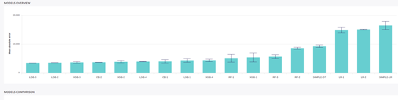
List of models of a version

You can quickly see :

performance of each model done , evaluated on the metrics you choose for this version
stability of each model ( represented with a small error bar ) computed on a cross validation of the trainset using the fold column provided

Simple models

The Provision Platform always produces what we sometimes call “simple models”, a linear regression and a Random Forest of only 5 depth, called simple-LR and simple DT. It is always a good idea to watch performance of these models against the most complex one and ask yourself if using them could be good enough for your problem.

Indeed, as they are very simple :

they can be implement in sql ( auto-generated code is even provided on the model analysis page )
they often are more explainable and are more accepted from the Business teams, are they are easier to understand and use.

As a data scientist, deciding to use a simple if-else instead of a complex Blend of Gradient Boosting if it solves the issue is within your purview!

On the experiment above, the :

LGB-3, XGB-4, and CB-2 look promising so we are going to have a closer look. Click on the model barplot to enter the detailed model analysis, CB-2 for example.

Here you have more detail about the models you select, like various metrics and the actual vs predicted Scatterplot.

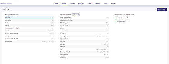
All the metrics of the model

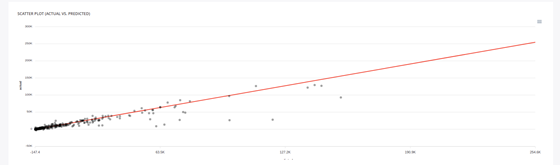
Predicted vs actual

You can download the Cross validation file if you want to run your own evaluation. The CB2 is quite good but if we look at the Scatterplot, we see that performance falls in the range from 40k to 80k. If we go to the LGB-3 page, we see a more stable performance.

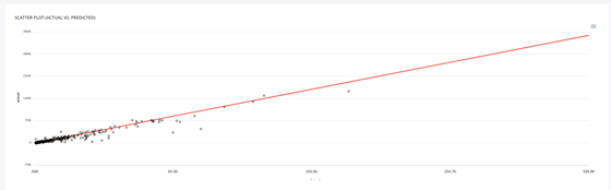
Predicted vs actual ( LGB-3 )

Evaluating a model is out of the scope of this guide but be aware that it is another step where you MUST involve your business team and explain each metrics and chart to them so you can choose the model that best solves their problem through group consensus.

The model analysis page is full of metrics to parse and you can run as many experiments as you want in order to find the model that fits the business problem the best.

After discussions with the LoB, we decided to keep the LGB-3 and the XGB-4, one because it performs well and the others because its performance is stable when evaluated on the holdout.

In order to refine this, we are now going to deploy both models and see how they perform in the real world.

Status

Task	Status	Output	Time spent
Data acquisition	Done	one trainset, one holdout	5mn
Feature engineering	Done	one engineered dataset with features, one holdout	20mn
Define the problem	Done	a metric to validate the models	1 week
Experiment	Done	~100 models	~20mn
Evaluate	Done	2 models selected with business team	1 week

Deploy

In this step two models will be deployed in order to test them on real data and usage. While deployed, their performance will be closely monitored for deciding if they are good for production grade utilisation.

Go to the “Deployment” section of your project and click on deploy a new experiment. Select LGB-3 as the main model and XGB-4 as a challenger in order to see which one performs best on real data.

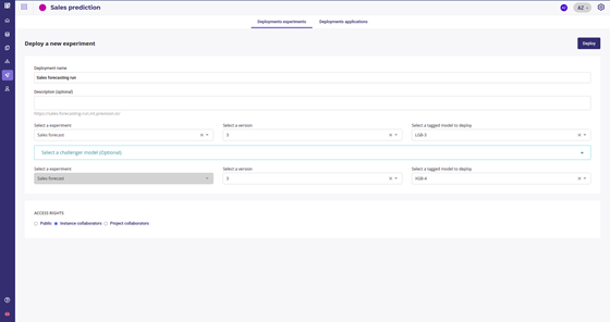
Set your main and challenger

The Main model will be used for prediction but each time you call it, a prediction will be done with the challenger model too and a chart will be generated so you can compare them.

Wait a few minutes to get :

a standalone webapp for a human user to test ( “Application link” url )
a batch predictor available for scheduling prediction
a REST API for calling the model from others software ( “Documentation API” link )

Set your main and challenger

That’s all. Your model can now be called from any client of your company and all its requests will be logged for further monitoring. Yet, in order to send predictions each week to the sales team, you need to schedule them.

Status

Task	Status	Output	Time spent
Data acquisition	Done	one trainset, one holdout	5mn
Feature engineering	Done	one engineered dataset with features, one holdout	20mn
Define the problem	Done	a metric to validate the models	1 week
Experiment	Done	~100 models	~20mn
Evaluate	Done	2 models selected with business team	1 week
Deploy	Done	Model available across the organization	5mn

Schedule

Once any model is deployed, it can be used to schedule prediction. First step is to insert it into a pipeline template and then create a new Schedule using this template.

Note that you need help from your IT team in this step, in order to define the name of the table where you will read the features from each week. You can use the same table that will be overwritten each week, for example “sales to predict” to read and “Sales predicted” to write, or a more complex naming scheme.

First you need to create two new assets :

a new datasource that will link to the Table where the IT team is going to put the features for prediction each week
a new exporter to push the result

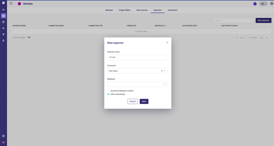
Create an exporter to push data to your crm

So you can use them in a new pipeline template with 3 nodes again:

Import from the datasource, where the datasource is the table with all the weekly features
a deployment prediction regression node
an export dataset node, that uses the exporter above

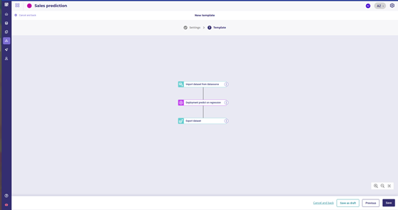
Template

Once you have your template, create a new Schedule based on it.

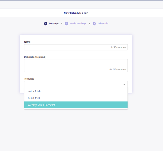
Use your template in a schedule run

Choose the Name of your deployment as the experiment deployment ID

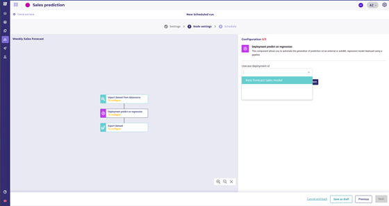
Use your template in a schedule run

And then, instead of the manual Trigger, use a periodic one, putting the configuration that fits your need the best ( here, a weekly prediction each Monday at 7:00 AM )

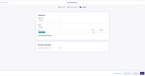
Scheduling a prediction each monday Morning

Click run and wait a few seconds. Your Prediction is now scheduled to run every Monday, from the table of “sales to predict” to the “Sales predicted” table of your databases.

Status

Task	Status	Output	Time spent
Data acquisition	Done	one trainset, one holdout	5mn
Feature engineering	Done	one engineered dataset with features, one holdout	20mn
Define the problem	Done	a metric to validate the models	1 week
Experiment	Done	~100 models	~20mn
Evaluate	Done	2 models selected with business team	1 week
Deploy	Done	Model available across the organization	5mn
Schedule	Done	Prediction in CRM each Monday at 09:00	20mn

Monitoring

Once a model is deployed, each call to it will be logged, being unit one or scheduled batch. You can track your model into the Deployments section of your project by clicking on a deployed experiment name in the list of experiments to access the deployment dashboard.

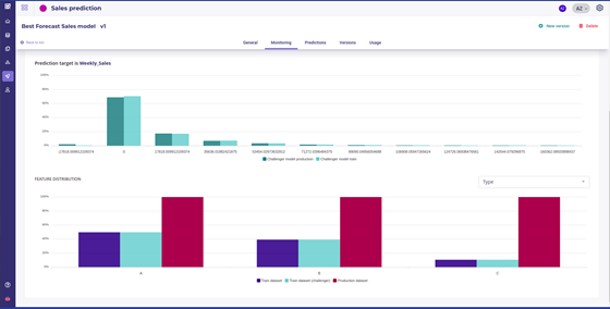
Train and production distribution

You can watch the features distribution of the trainset compared to the feature distribution seen in production and check the drift. Target distribution of the Main Model and Challenger model are shown side-by-side with those of the production in order to evaluate performance in a real application.

Under the monitoring/usage tab sit some SLA statistics about number of call average response time and errors.

By tracking all these indicators for a month or more, you can evaluate how your model lives in production and check that it behaves the way you expected while evaluating it in the experiment step.

Status

Task	Status	Output	Time spent
Data acquisition	Done	one trainset, one holdout	5mn
Feature engineering	Done	one engineered dataset with features, one holdout	20mn
Define the problem	Done	a metric to validate the models	1 week
Experiment	Done	~100 models	~20mn
Evaluate	Done	2 models selected with business team	1 week
Deploy	Done	Model available across the organization	5mn
Schedule	Done	Prediction in CRM each Monday at 09:00	20mn
Monitor	Done	Prediction in CRM each Monday at 09:00	1 month

Conclusion

In this guide, you saw how to complete the whole data science process in less than a morning and went from data to fully deployed model, shared across the company with full monitoring.

Using a tool to solve the technical issue of the data science, like finding the best model, deploying a model or importing the data, allows you to spend more time on what truly matters : talk with the Line of Business team to translate their problem to datascience configuration and metrics.

What is this Guide about ?

What’s in this guide ?

Starting point

Steps

Results

Data acquisition

Feature engineering

Define the problem

Experiment

Evaluate

Deploy

Schedule

Monitoring

Conclusion

NEED MORE INFORMATION?