It’s often quoted, “Data is the new oil” and as a data scientist, I clearly know the value of good data to train our model. However, we often face some problems with data:

  • Limited or no access because of confidentiality / governance requirements
  • Lack of sufficient quantity
  • It’s unbalanced and thus leads to biased models
  • … the list could go on and on.

In this guide, we will explore the usage and performance of synthetic data generation. If you want to try it by yourself you can:

Usage of synthetic Data

A common problem in the just about every  industry (telecom, banking, healthcare, etc.) is confidentiality of data. We want to build models using sensitive data while avoiding confidential or proprietary information.

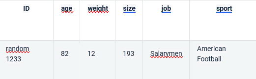
As an example, you may have a dataset in which each row is age, gender, size, weight, place of residence, etc. Even if data is anonymized by removing name or email, it’s often easy to find some particular person through their unique combination of features as in the following example:

A 30 year old man who lives near Cambridge, earns $30000 a month, whose wife is an engineer and subscribes to a sports magazine would be unique enough to know a lot about him, even without identity data. o no.

The second problem is lack of data or worse, a lack of data for some segment of the population that will then be disadvantaged by models.

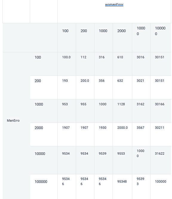
For example, let’s say that we have a dataset with 10000 men and 1000 women and we are using RMSE as the metric for our training. Let’s say for the sake of this article that every prediction for men has the same error manError and women have a womanError constant error.

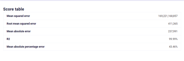
The Score of a model will be :

df['RMSE'] = ((10000*(df['manError']**2) + 1000*(df['womanError']**2))/(10000 + 1000))**.5

And the errors of each gender will be weighted as follows on the training metric :

We clearly see that making an error on the woman segment weighs much less on the optimized metric, as going from a 100 to 10000 woman error only goes from 100 to 3016 total error yet for men it goes from 100 to 9534 .

A goal of machine learning models is to find the minimum of given metrics.  A model trained on this data will advantage the men segment over the women segment. Of course, if we had the same number of men and women data, the error would be balanced and no bias toward a segment would occur. But adding more women data is not enough.  We cannot just copy and paste more rows, as it will lack diversity.

What we should do instead is add more “realistic” women data by sampling from the underlying distribution of each woman feature.


Weight distribution for some segment

Yet, if we just do that the naive way, this could happen :

(Note: of course retired women may play american football, yet weighing 12kg and playing american football when you are 82 years old is quite odd)

There are two pitfalls when generating fake data :

  • Assuming everything is a normal distribution and reducing a feature to its average and its deviation. In fact, most real world distribution is skewed
  • Not caring about joint probability distribution.

This is where a good synthetic Data Generator comes to the rescue.

Performance of synthetic Data Generator evaluation

Like every data science modelization, synthetic data generation needs some metric to measure performance of different algorithms. This metric should capture three expected outputs of synthetic data:

  • Distribution should “look like” real data
  • The joint probability distribution should look like the real one too (of course, someone who weighs 12kg should not be 1.93m tall, this criteria is sometimes call likelihood fitness )
  • Model performance should stay constant

Statistical properties of Generated Synthetic Data

The obvious way to generate synthetic data is to assume every feature follows a normal distribution, compute means and deviation, and generate data from gaussian distribution ( or discrete uniform distribution ) with the following statistics :

In python

nrm = pd.DataFrame()

for feat in ["price","sqft_living","sqft_lot","yr_built"]:
   stats=src.describe()[feat].astype(int)
   mu, sigma = stats['mean'], stats['std']
   s = np.random.normal(mu, sigma, len(dst))
   nrm[feat] = s.astype(int)

# For discrete Features
for feat in ["bedrooms","bathrooms"]:
   p_bath = (src.groupby(feat).count()/len(src))["price"]
   b=np.random.choice(p_bath.index, p=p_bath.values,size=len(dst))
   nrm[feat] = b

This approach leads to poor feature and joint distribution.

In the following plot, we show the distribution of features of a dataset (blue) , distribution of a synthetic dataset generated with a CTGAN in quick mode (orange, only 100 epoch for fitting ) and distribution of data assuming each feature is independant and follows a normal distribution (see code above).

For price, we see that generated data perfectly captures the distribution. It’s so good that we barely see the orange curve. Gaussian random data has the same mean and deviation as the original data but clearly does not fit the true data distribution.

For yr_built, the synthetic data generator (orange) struggles to perfectly capture the true distribution (blue) but it looks better than the average.

Price and bedrooms distribution

Below is the density chart for price, zoomed.

Zoom on price distribution

It’s more difficult to see joint distribution on this chart but we can draw a contour map to get a better view:

Original true Data Joint distribution of price and year constructed

Generated Data Joint distribution of same features. We see density start to reach those of real data

Independent random variable distribution; jointplot density is totally wrong

The same conclusion goes for other features as well. Random independent data do not fit distribution and joint distribution as effectively as properly generated data.

Each feature has its own distribution and distribution relative to others

Of course, better models than simple normal distribution do exist.

You can build kernel density estimation, gaussian mixture model or use other distribution than a normal. However,

But as you build more and more complex models, you soon will discover that you can use machine Learning  to do the job instead of looking manually for the best  distribution shape and parameters.
And that is where you start to use Generative Adversarial Network.

Generating good Synthetic Data

Like the prior image, Tabular data benefits from the usage of Generative Adversarial Networks with a Discriminator. In order to avoid the issue shown above, we can train a neural network on data whose input would be for each sample vector of:

  • discrete probability for each mode of categorical variable
  • probability of each mode of a a gaussian mixture model

The network is then tasked to generate a “fake sample” output and a Discriminator then tries to guess if this output comes from the Generator or from the true data.

By doing this, the Generator will learn both distribution and joint distribution between each feature, converging to a generator that outputs a sample as true as the real one.

The current best implementation of this idea is CTGAN that you can use on our Marketplace

Machine Learning efficiency

The best practical performance estimation of generated data is Machine Learning efficiency. We ran performance tests using our AI Management Platform with the optimal parameters (all models tried, hyper optimization and Blending of models) on 3 datasets with the same target :

  • Original dataset
  • Synthetic dataset fit on 800 epochs
  • Random Dataset with no joint probability

We expect that by using the AutoML feature, only data quality would change the performance.

Here are the results :

Modelization on true Data

Modelization on Synthetic Data

Modelisation on random independent data

We see that with CTGAN synthetic data, machine learning efficiency is preserved, which is not the case for independent data distribution.

Moreover, this efficiency is good even for segments of the original dataset, meaning you can generate synthetic samples for under-represented categories and keep their signal high enough to fix any bias in your dataset.

Going Further

You can read the original paper for CTGAN and find more here.

The CTGAN implementation is available on our Marketplace and you can test it with one of our public standard Dataset

Remember that synthetic data is very useful when you need to enforce data privacy or unbias a dataset. Training a Synthetic Data Generator for a few hours to build a generator that generates synthetic data should become part of your data science toolkit.


Arnold Zephir

About the author

Arnold Zephir

User advocacy