
In the previous article of our blog post series on machine learning metrics, we saw the difference between a metric and an objective function, and why metrics are important and how to choose a good one. In this article, we will focus on binary classification metrics. We provide below the links to others articles of this blog post.
- An introduction to Machine Learning metrics
- Binary Classification metrics
- Regression metrics
- Multi Classification metrics
Introduction
Classification refers to predictive modeling problems that involve predicting a class label. To evaluate the models, different types of metrics can be used. In binary classification, these metrics can be decomposed into three categories:
- metrics whose objective is to order the instances like AUC,
- metrics whose objective is to offer the most qualitative probability possible like log loss,
- metrics whose objective is to maximize the final decision like accuracy or F1 score.
In this article, you will discover how to calculate metrics for binary classification predictive modeling projects.
I would like to thank Abishek Takhur for allowing us to reuse the implementation code for the metrics discussed in this article. We invite you to read the excellent book Approaching (Almost) Any Machine Learning Problem.
To explain the metrics discussed in this article, we first need to introduce the concepts of confusion, precision and recall matrix.
Confusion Matrix
The confusion matrix is a performance measurement for machine learning classification in both binary and multi-class classification. It compares the predicted classes by the models to the ground truth classes. However, most machine learning tools return the probability of belonging to each class (example: 0.33) and not the class label (example predicted class = 0). Therefore, there is a need to convert these probabilities into class labels.
How to convert Probabilities to Class Labels?
To convert probabilities to class labels, a threshold can be defined. Based on the latter, each object will be assigned to the class with the probability above the threshold. In Provision.io, in order to obtain an optimal threshold, several ones are tested. The optimal threshold is obtained by maximizing F1 Score.
True Positive / True Negative / False Positive / False Negative
Once the conversion is done, the confusion matrix is obtained from the following table.
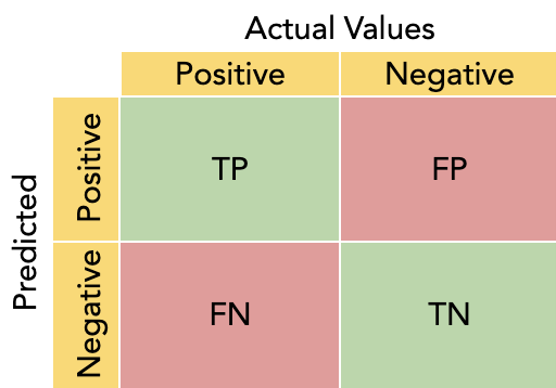
Confusion matrix [source]
Columns in the confusion matrix table represent the actual values of the target and rows the predicted value of the target by the classification model. TP (True Positive) corresponds to the number of predicted positive classes which are actually positive. Similarly to TP, TN (True Negative) corresponds to the number of predicted negative classes which are actually negative. FP (False Positive or Type 1 error) corresponds to the number of predicted positive classes which are actually negative. FN (False Negative or Type 2 error) corresponds to the number of predicted negative classes which are actually positive. This is usually the error we need to decrease the most.
The confusion matrix can be seen as an overview of the model’s predictions. We can easily read the percentage of correct predictions (diagonal) and of incorrect ones (anti-diagonal).
Below is the implementation in python of the calculation of the confusion matrix.
def true_positive(y_true, y_pred):
 """
 Function to calculate True Positives
 :param y_true: list of true values
 :param y_pred: list of predicted values
 :return: number of true positives
 """
 # initialize
 tp = 0
 for yt, yp in zip(y_true, y_pred):
 if yt == 1 and yp == 1:
 tp += 1
 return tp
def true_negative(y_true, y_pred):
 """
 Function to calculate True Negatives
 :param y_true: list of true values
 :param y_pred: list of predicted values
 :return: number of true negatives
 """
 # initialize
 tn = 0
 for yt, yp in zip(y_true, y_pred):
 if yt == 0 and yp == 0:
 tn += 1
 return tn
def false_positive(y_true, y_pred):
 """
 Function to calculate False Positives
 :param y_true: list of true values
 :param y_pred: list of predicted values
 :return: number of false positives
 """
 # initialize
Approaching (Almost) Any Machine Learning Problem - Abhishek Thakur
35
 fp = 0
 for yt, yp in zip(y_true, y_pred):
 if yt == 0 and yp == 1:
 fp += 1
 return fp
def false_negative(y_true, y_pred):
 """
 Function to calculate False Negatives
 :param y_true: list of true values
 :param y_pred: list of predicted values
 :return: number of false negatives
 """
 # initialize
 fn = 0
 for yt, yp in zip(y_true, y_pred):
 if yt == 1 and yp == 0:
 fn += 1
 return fn
Precision / Recall
Precision (also called positive predictive value) is the fraction of relevant instances among the retrieved instances, while recall (also known as sensitivity) is the fraction of relevant instances that were retrieved. Both precision and recall are therefore based on relevance.
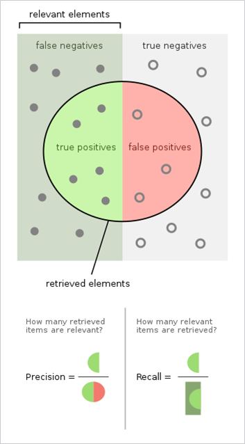
Precision / Recall definitions [source]
Below is the implementation in python of the calculation of the precision and the recall.
def precision(y_true, y_pred):
"""
Function to calculate precision
:param y_true: list of true values
:param y_pred: list of predicted values
:return: precision score
"""
tp = true_positive(y_true, y_pred)
fp = false_positive(y_true, y_pred)
precision = tp / (tp + fp)
return precision

def recall(y_true, y_pred):
"""
Function to calculate recall
:param y_true: list of true values
:param y_pred: list of predicted values
:return: recall score
"""
tp = true_positive(y_true, y_pred)
fn = false_negative(y_true, y_pred)
recall = tp / (tp + fn)
return recall
All the terms explained below will be used in the calculation of the following metrics.
AUC
AUC means Area Under the Receiver Operating Characteristic Curve.
This metric is used to evaluate how well a binary classification model is able to distinguish between true positives and false positives. The AUC score represents the degree or measure of separability. It tells how much the model is capable of distinguishing between classes. An AUC of 1 indicates a perfect classifier, while an AUC of .0.5 indicates a poor classifier whose performance is no better than random guessing. The AUC bears its name because it is represented in graphic form as below
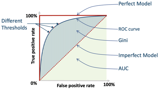
Example of ROC CURVE [source]
from sklearn import metrics
metrics.roc_auc_score(y_true, y_pred)
GINI
The GINI score is an adjustment to the AUC so that a perfectly random model scores 0 and a reversing model has a negative sign.
from sklearn import metrics
Gini = 2 * metrics.roc_auc_score(y_true, y_pred) - 1
Log loss
The logarithmic loss metric can be used to evaluate the performance of a binomial classifier. Unlike the AUC which looks at how well a model can classify a binary target, the log loss evaluates how close a model’s predicted values (uncalibrated probability estimates) are to the actual target value. For example, does a model tend to assign a high predicted value like 0.80 for the positive class, or does it show a poor ability to recognize the positive class and assign a lower predicted value like 0.50?
The log loss can be any value greater than or equal to 0, with 0 meaning that the model correctly assigns a probability of 0% or 100%.
The log loss equation is defined as follows:
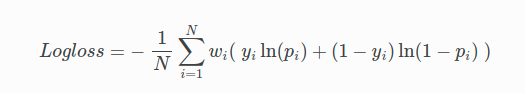
Where:
- N is the total number of rows (observations) of your corresponding dataframe.
- w is the per row user-defined weight (defaults is 1).
- p is the predicted value (uncalibrated probability) assigned to a given row (observation).
- y is the actual target value.
Below is the implementation in python of the calculation of the log loss.
import numpy as np
def log_loss(y_true, y_proba):
 """
 Function to calculate log loss
 :param y_true: list of true values
 :param y_proba: list of probabilities for 1
 :return: overall log loss
 """
 # define an epsilon value
 # this can also be an input
 # this value is used to clip probabilities
 epsilon = 1e-15
 # initialize empty list to store
 # individual losses
 loss = []
 # loop over all true and predicted probability values
 for yt, yp in zip(y_true, y_proba):
 # adjust probability
 # 0 gets converted to 1e-15
 # 1 gets converted to 1-1e-15
 # Why? Think about it!
 yp = np.clip(yp, epsilon, 1 - epsilon)
 # calculate loss for one sample
 temp_loss = - 1.0 * (
 yt * np.log(yp)
 + (1 - yt) * np.log(1 - yp)
 )
 # add to loss list
 loss.append(temp_loss)
 # return mean loss over all samples
 return np.mean(loss)
Accuracy
In binary classification, the accuracy score is the number of correct predictions over the number of observations:
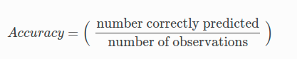
This metric is not recommended when your target is imbalanced. Indeed, let’s take the example of a churn problem with a positive target rate of 1%. A model that predicts “no churn” for all observations will have an accuracy level of 99% which is great but unnecessary for identifying churners. In the case of imbalance classes, we recommend the use of the AUC metric.
Below is the implementation in python of the calculation of the accuracy metric.
def accuracy(y_true, y_pred):
"""
Function to calculate accuracy
:param y_true: list of true values
:param y_pred: list of predicted values
:return: accuracy score
"""
# initialize a simple counter for correct predictions
correct_counter = 0
# loop over all elements of y_true
# and y_pred "together"
for yt, yp in zip(y_true, y_pred):
if yt == yp:
# if prediction is equal to truth, increase the counter
correct_counter += 1
# return accuracy
# which is correct predictions over the number of samples
return correct_counter / len(y_true)
Error Rate
Error rate is deduced from the previous Accuracy metric as follows:
Error rate = 1 – Accuracy.
Some users of the Provision.io platform prefer to display the accuracy rate over the error one. It is very dependent on the use case. For example, for a problem of predictive maintenance, we will try to minimize the error rate.
As for the previous metric, this metric should not be used in the case of imbalance classes.
def error_rate(y_true, y_pred):
"""
Function to calculate accuracy
:param y_true: list of true values
:param y_pred: list of predicted values
:return: accuracy score
"""
# initialize a simple counter for correct predictions
correct_counter = 0
# loop over all elements of y_true
# and y_pred "together"
for yt, yp in zip(y_true, y_pred):
if yt == yp:
# if prediction is equal to truth, increase the counter
correct_counter += 1
# return accuracy
# which is correct predictions over the number of samples
return 1 - (correct_counter / len(y_true))
F1
The F1 score provides a measure of how well a binary classifier can classify positive cases (given a threshold value). The F1 score is calculated from the harmonic mean of the precision and recall. An F1 score of 1 means both precision and recall are perfect and the model correctly identified all the positive cases and didn’t mark a negative case as a positive case. If either precision or recall are very low it will be reflected with a F1 score closer to 0.
The F1 equation is given as follows:
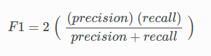
F1 Equation Formula
Where:
- precision is the positive observations (true positives) the model correctly identifies from all the observations it labeled as positive (the true positives + the false positives).
- recall is the positive observations (true positives) the model correctly identified from all the actual positive cases (the true positives + the false negatives).
There are several versions of the F1 score depending on the expected granularity.
- micro: Calculate metrics globally by counting the total true positives, false negatives and false positives.
- macro: Calculate metrics for each label, and find their unweighted mean. This does not take label imbalance into account.
- weighted: Calculate metrics for each label, and find their average weighted by support (the number of true instances for each label). This alters ‘macro’ to account for label imbalance; it can result in an F-score that is not between precision and recall.
Below is the implementation in python of the calculation of true positive, true negative, false positive and false negative.
def true_positive(y_true, y_pred):
 """
 Function to calculate True Positives
 :param y_true: list of true values
 :param y_pred: list of predicted values
 :return: number of true positives
 """
 # initialize
 tp = 0
 for yt, yp in zip(y_true, y_pred):
 if yt == 1 and yp == 1:
 tp += 1
 return tp
def true_negative(y_true, y_pred):
 """
 Function to calculate True Negatives
 :param y_true: list of true values
 :param y_pred: list of predicted values
 :return: number of true negatives
 """
 # initialize
 tn = 0
 for yt, yp in zip(y_true, y_pred):
 if yt == 0 and yp == 0:
 tn += 1
 return tn
def false_positive(y_true, y_pred):
 """
 Function to calculate False Positives
 :param y_true: list of true values
 :param y_pred: list of predicted values
 :return: number of false positives
 """
 # initialize
 fp = 0
 for yt, yp in zip(y_true, y_pred):
 if yt == 0 and yp == 1:
 fp += 1
 return fp
def false_negative(y_true, y_pred):
 """
 Function to calculate False Negatives
 :param y_true: list of true values
 :param y_pred: list of predicted values
 :return: number of false negatives
 """
 # initialize
 fn = 0
 for yt, yp in zip(y_true, y_pred):
 if yt == 1 and yp == 0:
 fn += 1
 return fn

import numpy as np
def macro_precision(y_true, y_pred):
 """
 Function to calculate macro averaged precision
 :param y_true: list of true values
 :param y_pred: list of predicted values
 :return: macro precision score
 """

 # find the number of classes by taking
 # length of unique values in true list
 num_classes = len(np.unique(y_true))

 # initialize precision to 0
 precision = 0

 # loop over all classes
 for class_ in range(num_classes):

 # all classes except current are considered negative
 temp_true = [1 if p == class_ else 0 for p in y_true]
 temp_pred = [1 if p == class_ else 0 for p in y_pred]

 # calculate true positive for current class
 tp = true_positive(temp_true, temp_pred)

 # calculate false positive for current class
 fp = false_positive(temp_true, temp_pred)

 # calculate precision for current class
 temp_precision = tp / (tp + fp)

 # keep adding precision for all classes
 precision += temp_precision
 # calculate and return average precision over all classes
 precision /= num_classes
 return precision

import numpy as np
def micro_precision(y_true, y_pred):
 """
 Function to calculate micro averaged precision
 :param y_true: list of true values
 :param y_pred: list of predicted values
 :return: micro precision score
 """

 # find the number of classes by taking
 # length of unique values in true list
 num_classes = len(np.unique(y_true))

 # initialize tp and fp to 0
 tp = 0
 fp = 0

 # loop over all classes
 for class_ in range(num_classes):
 # all classes except current are considered negative
 temp_true = [1 if p == class_ else 0 for p in y_true]
 temp_pred = [1 if p == class_ else 0 for p in y_pred]

 # calculate true positive for current class
 # and update overall tp
 tp += true_positive(temp_true, temp_pred)

 # calculate false positive for current class
 # and update overall tp
 fp += false_positive(temp_true, temp_pred)

 # calculate and return overall precision
 precision = tp / (tp + fp)
 return precision


from collections import Counter
import numpy as np
def weighted_precision(y_true, y_pred):
 """
 Function to calculate weighted averaged precision
 :param y_true: list of true values
 :param y_pred: list of predicted values
 :return: weighted precision score
 """

 # find the number of classes by taking
 # length of unique values in true list
 num_classes = len(np.unique(y_true))

 # create class:sample count dictionary
 # it looks something like this:
 # {0: 20, 1:15, 2:21}
 class_counts = Counter(y_true)

 # initialize precision to 0
 precision = 0

 # loop over all classes
 for class_ in range(num_classes):
 # all classes except current are considered negative
 temp_true = [1 if p == class_ else 0 for p in y_true]
 temp_pred = [1 if p == class_ else 0 for p in y_pred]

 # calculate tp and fp for class
 tp = true_positive(temp_true, temp_pred)
 fp = false_positive(temp_true, temp_pred)

 # calculate precision of class
 temp_precision = tp / (tp + fp)

 # multiply precision with count of samples in class
 weighted_precision = class_counts[class_] * temp_precision

 # add to overall precision
 precision += weighted_precision
 # calculate overall precision by dividing by
 # total number of samples
 overall_precision = precision / len(y_true)
 return overall_precision
F0.5
The F0.5 score is the weighted harmonic mean of the precision and recall (given a threshold value). Unlike the F1 score, which gives equal weight to precision and recall, the F0.5 score gives more weight to precision than to recall. More weight should be given to precision for cases where False Positives are considered worse than False Negatives. For example, if your use case is to predict which products you will run out of, you may consider False Positives worse than False Negatives. In this case, you want your predictions to be very precise and only capture the products that will definitely run out. If you predict a product will need to be restocked when it actually doesn’t, you incur cost by having purchased more inventory than you actually need.
The F0.5 equation is given as follows:
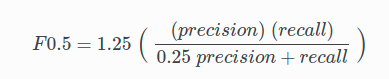
Where:
- precision is the positive observations (true positives) the model correctly identifies from all the observations it labeled as positive (the true positives + the false positives).
- recall is the positive observations (true positives) the model correctly identified from all the actual positive cases (the true positives + the false negatives).
from sklearn.metrics import fbeta_score
def f05score(y_true, y_pred):
    return fbeta_score(y_true, y_pred,beta=0.5)
F2
The F2 score is the weighted harmonic mean of the precision and recall (given a threshold value). Unlike the F1 score, which gives equal weight to precision and recall, the F2 score gives more weight to recall than to precision. More weight should be given to recall for cases where False Negatives are considered worse than False Positives. For example, if your use case is to predict which customers will churn, you may consider False Negatives worse than False Positives. In this case, you want your predictions to capture all of the customers that will churn. Some of these customers may not be at risk for churning, but the extra attention they receive is not harmful. More importantly, no customers actually at risk of churning have been missed.
The F2 score is defined by the following equation:
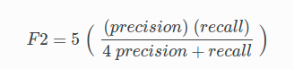
Where:
- precision is the positive observations (true positives) the model correctly identified from all the observations it labeled as positive (the true positives + the false positives).
- recall is the positive observations (true positives) the model correctly identified from all the actual positive cases (the true positives + the false negatives).
In the literature, there are also F3 and F4 metrics which give even more weight to recall. For all practical purposes, these metrics are also implemented in Provision.io.
from sklearn.metrics import fbeta_score
def f2score(y_true, y_pred):
    return fbeta_score(y_true, y_pred,beta=2)
MCC
MCC stands for Means Matthews Correlation Coefficient. It represents the confusion matrix of a
model as a single number by combining the true positives, false positives, true negatives, and
false negatives using the equation described below.
The same process to determine an optimal threshold for the conversion of probabilities to class labels is used to find the maximal value MCC. By choosing this metric, Provision.io goal is to continue increasing this maximum MCC.
Unlike metrics like Accuracy, MCC is a good scorer to use when the target variable is imbalanced. In the case of imbalanced data, high Accuracy can be found by predicting the majority class. Metrics like Accuracy and F1 can be misleading, especially in the case of imbalanced data, because they do not consider the relative size of the four confusion matrix categories. MCC, on the other hand, takes the proportion of each class into account. The MCC value ranges from -1 to 1 where -1 indicates a classifier that predicts the opposite class from the actual value, 0 means the classifier does no better than random guessing, and 1 indicates a perfect classifier.
MCC is defined as follows:
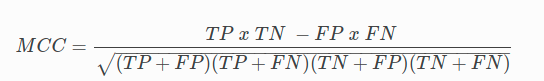
Where:
- TP = True Positive,
- TN = True Negative,
- FP = False Positive,
- FN = False Negative. (if you have the slightest doubt about the understanding of these terms, I invite you to review the confusion matrix paragraph)
from sklearn.metrics import matthews_corrcoef
def mcc(y_true, y_pred):
      return matthews_corrcoef(y_true, y_pred)
service@provision.guru
The lift @ k metric measures the overconcentration obtained by the model at k%.
Indeed, for certain issues, in particular to operate marketing actions, for cross sell or churn issues, it is not a question of maximizing the order of all instances, as in the case of the AUC metric, but to maximize a fraction (k%) of the total population.
For example: telemarketing call for the 5% top scores, sending a sponsorship code for the 20% top scores, …
At Provision.io, the lift can be represented by decile, i.e. by dividing the population into increments of 10%, as shown in the following graph.
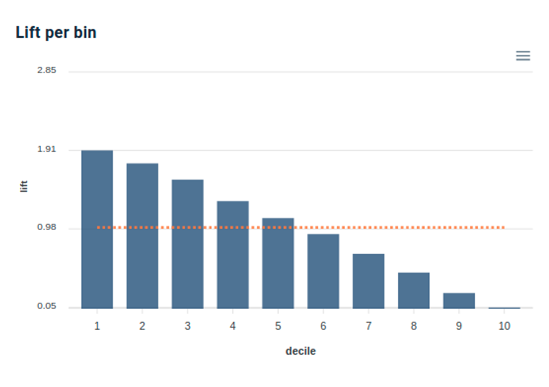
Lift per decile in Provision.io
from scikitplot.metrics import plot_lift_curve
fig, ax = plt.subplots()
plot_lift_curve(y_true, y_pred, ax=ax)
The following table summarizes the binary classification metrics discussed in this article.
|
|
|
| Provision.io Notation |
| |||
METRIC | Range | Lower is better | Weights accepted | 3 STARS | 2 STARS | 1 STAR | 0 STAR | Tips |
AUC | 0 – 1 | False | True | ]0.85 ; 1] | ]0.65 ; 0.85] | ]0.5 ; 0.65] | [0 ; 0.5] | Optimizes sort order of predictions |
LOGLOSS | 0 – ∞ | True | True | [0 ; 0.223[ | [0.223 ; 0.693[ | [0.693 ; +inf[ |
| Optimizes probabilities |
ERROR RATE | 0 – 1 | True | True | [0 ; 0.125[ | [0.125 ; 0.25[ | [0.25 ; +inf[ |
| Highly interpretable |
Accuracy | 0 – 1 | False | True | ]0.875 ; 1] | ]0.75 ; 0.875] | ]0.5 ; 0.75] | [0: 0.5] | Highly interpretable |
F1 | 0 – 1 | False | True | ]0.85 ; 1] | ]0.65 ; 0.85] | ]0.5 ; 0.65] | [0 ; 0.5] | Equal weight on precision and recall |
MCC | 0 – 1 | False | True | ]0.9 ; 1] | ]0.7 ; 0.9] | ]0.5 ; 0.7] | [-1 ; 0.5] | All classes are equally weighted |
Gini | 0 – 1 | False | True | ]0.85 ; 1] | ]0.65 ; 0.85] | ]0.5 ; 0.65] | [0 ; 0.5] |
|
F05 | 0 – 1 | False | True | ]0.85 ; 1] | ]0.65 ; 0.85] | ]0.5 ; 0.65] | [0 ; 0.5] |
|
F2 | 0 – 1 | False | True | ]0.85 ; 1] | ]0.65 ; 0.85] | ]0.5 ; 0.65] | [0 ; 0.5] | More weight on recall, less weight on precision |
F3 | 0 – 1 | False | True | ]0.85 ; 1] | ]0.65 ; 0.85] | ]0.5 ; 0.65] | [0 ; 0.5] | More More weight on recall, less weight on precision |
F4 | 0 – 1 | False | True | ]0.85 ; 1] | ]0.65 ; 0.85] | ]0.5 ; 0.65] | [0 ; 0.5] | More More More weight on recall, less weight on precision |
0 – ∞ | False | True | ]1 + 7 * (1-k) ; 1] | ]1 + 3 * (1-k) ; 1 + 7 * (1-k) ] | ]1 + 1 * (1-k) ; 1 + 3 * (1-k) ] | [0 ; 1 + 1 * (1-k)] | particularly useful when you want to maximize the lift on the X% top scores | |
Binary Classification metrics summary table
Conclusion
In this article, we introduced binary classification metrics that can be used to evaluate the performance of machine learning models. We discussed:
- the main binary classification metrics definitions, formula,
- their code implementation in Python,
- in which situations are they used,
- a summary table of these metrics
It should be noted that the metrics presented in this article are provided in our end-to-end machine learning platform Provision.io. A free trial can be found here.