
So far in this blog post series, we discussed the importance of choosing metrics for machine learning models, their importances and presented common metrics used in binary classification. In this article, we present common metrics that can be used to evaluate regression tasks.
To access the other articles, click below on the subject that interests you:
- An introduction to Machine Learning metrics
- Binary Classification metrics
- Regression metrics
- Multi Classification metrics
Introduction
Regression refers to predictive modeling problems that involve predicting a numeric value. It is different from classification that involves predicting a class label. Unlike classification, you cannot use classification accuracy to evaluate the predictions made by a regression model.
Instead, you must use error metrics specifically designed for evaluating predictions made on regression problems.
In this article, you will discover how to calculate error metrics for regression predictive modeling projects.
I would like to thank Abishek Takhur for allowing us to reuse the implementation code for the metrics discussed in this article. We invite you to read the excellent book Approaching (Almost) Any Machine Learning Problem.
Mean Square Error (MSE)
Mean Square Error (MSE) is defined as Mean or Average of the square of the difference between actual and estimated values. It measures the average of the squares of the errors or deviations. MSE takes the distances from the points to the regression line (these distances are the “errors”) and squaring them to remove any negative signs. The MSE score incorporates both the variance and the bias of the predictor. It also gives more weight to larger differences. The bigger the error, the more it is penalized.
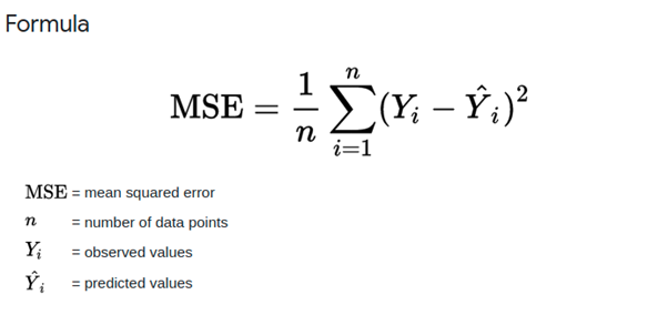
MSE Formula
def mean_squared_error(y_true, y_pred):
 """
 This function calculates mse
 :param y_true: list of real numbers, true values
 :param y_pred: list of real numbers, predicted values
 :return: mean squared error
 """
 # initialize error at 0
 error = 0
 # loop over all samples in the true and predicted list
 for yt, yp in zip(y_true, y_pred):
 # calculate squared error
 # and add to error
 error += (yt - yp) ** 2
 # return mean error
 return error / len(y_true)
Root Mean Square Error (RMSE)
The Root mean squared error (RMSE) is the square root of the mean of the square of all of the errors. The use of RMSE is very common, and it is considered an excellent general-purpose error metric for numerical predictions.
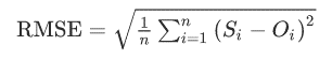
where:
- Oi are the observations,
- Si predicted values of a variable,
- n the number of observations available for analysis.
The RMSE score is a good measure of accuracy, but only to compare prediction errors of different models or model configurations for a particular variable and not between variables, as it is scale-dependent.
def root_mean_squared_error(y_true, y_pred):
 """
 This function calculates rmse
 :param y_true: list of real numbers, true values
 :param y_pred: list of real numbers, predicted values
 :return: root mean squared error
 """
 # initialize error at 0
 error = 0
 # loop over all samples in the true and predicted list
 for yt, yp in zip(y_true, y_pred):
 # calculate squared error
 # and add to error
 error += (yt - yp) ** 2
 # return mean error
 return np.sqrt(error / len(y_true))
Root Mean Square Logarithmic Error (RMSLE)
The RMSLE measures the ratio between actual and predicted. It is the Root Mean Squared Error of the log-transformed predicted and log-transformed actual values. RMSLE adds 1 to both actual and predicted values before taking the natural logarithm to avoid taking the natural log of possible 0 (zero) values.
In case of RMSLE, you take the log of the predictions and actual values. So basically, what changes is the variance that you are measuring. I believe RMSLE is usually used when you don’t want to penalize huge differences in the predicted and the actual values when both predicted and true values are huge numbers.
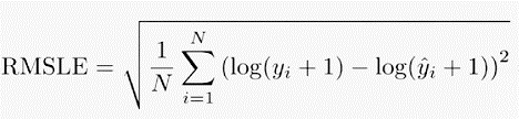
where:
- yi are the real values,
- ŷi predicted values of a variable,
- n the number of observations available for analysis.
import numpy as np
def root_mean_squared_log_error(y_true, y_pred):
 """
 This function calculates msle
 :param y_true: list of real numbers, true values
 :param y_pred: list of real numbers, predicted values
 :return: mean squared logarithmic error """
 # initialize error at 0
 error = 0
 # loop over all samples in true and predicted list
 for yt, yp in zip(y_true, y_pred):
 # calculate squared log error
 # and add to error
 error += (np.log(1 + yt) - np.log(1 + yp)) ** 2
 # return mean error
 return np.sqrt(error / len(y_true))
Root Mean Square Percentage Error (RMSPE)
The RMSPE, which is mostly used as an advanced forecasting metric, is defined by the following equation:
where:
- yi are the observations,
- ŷi predicted values of a variable,
- n the number of observations available for analysis.
def root_mean_squared_percentage_error(y_true, y_pred):
 """
 This function calculates rmse
 :param y_true: list of real numbers, true values
 :param y_pred: list of real numbers, predicted values
 :return: root mean squared percentage error
 """
 # initialize error at 0
 error = 0
 # loop over all samples in the true and predicted list
 for yt, yp in zip(y_true, y_pred):
 # calculate squared error
 # and add to error
 error += ((yt - yp)/yt) ** 2
 # return mean error
 return np.sqrt(error / len(y_true))
Mean Absolute Error (MAE)
The MAE score measures the average magnitude of the errors in a set of predictions, without considering their direction. It’s the average over the test sample of the absolute differences between prediction and actual observation where all individual differences have equal weight.
The mean absolute error uses the same scale as the data. This is known as a scale-dependent accuracy measure and, therefore, cannot be used to make comparisons between series using different scales.
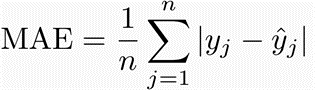
where:
- yj are the observations,
- ŷj predicted values of a variable,
- n the number of observations available for analysis.
import numpy as np
def mean_absolute_error(y_true, y_pred):
 """
 This function calculates mae
 :param y_true: list of real numbers, true values
 :param y_pred: list of real numbers, predicted values
 :return: mean absolute error
 """
 # initialize error at 0
 error = 0
 # loop over all samples in the true and predicted list
 for yt, yp in zip(y_true, y_pred):
 # calculate absolute error
 # and add to error
 error += np.abs(yt - yp)
 # return mean error
 return error / len(y_true)
Mean Absolute Percentage Error (MAPE)
The MAPE score measures the accuracy of a forecasting method in statistics, for example in trend estimation. It is also used as a loss function for regression problems in machine learning. The MAPE usually expresses accuracy as a percentage.
From Wikipedia, although the concept of MAPE sounds very simple and convincing, it has major drawbacks in practical application, and there are many studies on shortcomings and misleading results from MAPE.
- It cannot be used if there are zero values (which happens frequently in demand data for example) because there would be a division by zero.
- For forecasts which are too low the percentage error cannot exceed 100%, but for forecasts which are too high there is no upper limit to the percentage error.
- MAPE puts a heavier penalty on negative errors than on positive errors. As a consequence, when MAPE is used to compare the accuracy of prediction methods it is biased in that it will systematically select a method whose forecasts are too low. This little-known but serious issue can be overcome by using an accuracy measure based on the logarithm of the accuracy ratio (the ratio of the predicted to actual value). This approach leads to superior statistical properties and leads to predictions which can be interpreted in terms of the geometric mean.
To overcome these issues with MAPE, there are some other measures proposed in literature like the Symmetric Mean Absolute Percentage Error (SMAPE) presented later.
import numpy as np
def mean_abs_percentage_error(y_true, y_pred):
 """
 This function calculates MAPE
 :param y_true: list of real numbers, true values
 :param y_pred: list of real numbers, predicted values
 :return: mean absolute percentage error
 """
 # initialize error at 0
 error = 0
 # loop over all samples in true and predicted list
 for yt, yp in zip(y_true, y_pred):
 # calculate percentage error
 # and add to error
 error += np.abs(yt - yp) / yt
 # return mean percentage error
 return error / len(y_true)
Median Absolute Error (MedAE)
Median absolute error output is a non-negative floating point with an optimal value corresponding to 0. The median absolute error is particularly interesting because it is robust to outliers. The loss is calculated by taking the median of all absolute differences between the target and the prediction. If ŷ is the predicted value of the ith sample and yi is the corresponding true value, then the median absolute error estimated over n samples is defined as follows:
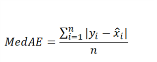
Where:
- X̂i is the median of the sample
- yi predictions
- n is total number of observations
import numpy as np
def median_absolute_error(y_true, y_pred):
    """Median absolute error regression loss.
    Median absolute error output is non-negative floating point. The best value
    is 0.0. Read more in the :ref:`User Guide <median_absolute_error>`.
    Parameters
    ----------
    y_true : array-like of shape = (n_samples) or (n_samples, n_outputs)
        Ground truth (correct) target values.
    y_pred : array-like of shape = (n_samples) or (n_samples, n_outputs)
    Returns
        weighted average of all output errors is returned.
    """
    return np.median(np.abs(y_pred - y_true), axis=0)
Symmetric Mean Absolute Percentage Error (SMAPE)
SMAPE means Symmetric Mean Absolute Percentage Error. This metric is an accuracy measure based on percentage (or relative) errors.
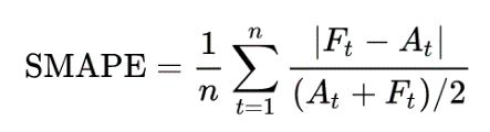
Where:
- Ai is the actual value
- Fi is the forecast value
- n is total number of observations
In contrast to the mean absolute percentage error, SMAPE has both a lower bound and an upper bound. Indeed, the formula above provides a result between 0% and 200%. However a percentage error between 0% and 100% is much easier to interpret.
A limitation to SMAPE is that if the actual value or forecast value is 0, the value of error will boom up to the upper-limit of error. (200% for the first formula and 100% for the second formula).
import numpy as np

def smape(y_true, y_pred):
    return 1/len(y_true) * np.sum(2 * np
R2 (R squared)
R² helps us to know how good our regression model is compared to a very simple model that just predicts the mean value of target from the train set as predictions.
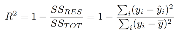
Where:
- SS RES term shows the sum of the Square of the distance between the actual point and the predicted point in the best-fit line.
- SS TOT term shows the sum of the Square of the distance between the actual point and the mean of all the points in the mean line.
- yi are the observations,
- ŷi predicted values,
mean values
import numpy as np
def r2(y_true, y_pred):
 """
 This function calculates r-squared score
 :param y_true: list of real numbers, true values
 :param y_pred: list of real numbers, predicted values
 :return: r2 score
 """

 # calculate the mean value of true values
 mean_true_value = np.mean(y_true)

 # initialize numerator with 0
 numerator = 0
 # initialize denominator with 0
 denominator = 0

 # loop over all true and predicted values
 for yt, yp in zip(y_true, y_pred):
 # update numerator
 numerator += (yt - yp) ** 2
 # update denominator
 denominator += (yt - mean_true_value) ** 2
 # calculate the ratio
 ratio = numerator / denominator
 # return 1 - ratio
 return 1 - ratio
Regression metrics summary table
|
|
|
| Provision.io Notation |
|
| |||
Metric | Range | Lower is better | Weights accepted | 3 Stars | 2 Stars | 1 Star | 0 Star | Sensitive to Outliers | Tips |
MSE | 0 – ∞ | True | True | [0 ; 0.01 * VAR[ | [0.01 * VAR ; 0.1 * VAR[ | [0.1 * VAR ; VAR [ | [VAR ; +inf [ | Yes |
|
RMSE | 0 – ∞ | True | True | [0 ; 0.1 * STD[ | [0.1 * STD ; 0.3 * STD[ | [0.3 * STD ;STD[ | [STD ; +inf [ | Yes |
|
MAE | 0 – ∞ | True | True | [0 ; 0.1 * STD[ | [0.1 * STD ; 0.3 * STD[ | [0.3 * STD ;STD[ | [STD ; +inf [ | No |
|
MAPE | 0 – ∞ | True | True | [0 ; 0.1[ | [0.1 ; 0.3[ | [0.3 ; 1[ | [1 ; +inf[ | No | Use when target values are across different scales |
RMSLE | 0 – ∞ | True | True | [0 ; 0.095[ | [0.095 ; 0.262[ | [0.262 ; 0.693[ | [0.693 ; +inf[ | Yes |
|
RMSPE | 0 – ∞ | True | True | [0 ; 0.1[ | [0.1 ; 0.3[ | [0.3 ; 1[ | [1 ; +inf[ | Yes | Use when target values are across different scales |
SMAPE | 0 – ∞ | True | True | [0 ; 0.1[ | [0.1 ; 0.3[ | [0.3 ; 1[ | [1 ; +inf[ | No | Use when target values are close to 0 |
R2 | -∞ – 1 | False | True | ]0.9 ; 1] | ]0.7 ; 0.9] | ]0.5 ; 0.7] | ]-inf ; 0.5] | No | Use when you want performance scaled between 0 and 1 |
Conclusion
We have introduced regression metrics, those implemented in Provision.io.
In this article we have seen:
- the main regression metrics,
- their code implementation in Python
- in which situations are they used
- a summary table of these metrics