
In this blog post series, we are going to explore Machine Learning metrics, their impact on a model and how they can have a critical importance from a business user perspective.
To access the other articles, click below on the subject that interests you:
- An introduction to Machine Learning metrics
- Binary classification metrics
- Regression metrics
- Multi Classification metrics
Introduction
Multi-class classification refers to classification challenges in machine learning that involve more than two classes. When evaluating and comparing machine learning algorithms on multi class targets, performance metrics are extremely valuable. Many measures can be used to evaluate a multi-class classifier’s performance. These metrics prove beneficial at many stages of the development process, such as comparing the performance of two different models or analyzing the behavior of the same model by changing various parameters. In this post, we go through a list of the most often used multi-class metrics, their benefits and drawbacks, and how they can be employed in the building of a classification model.
I would like to thank Abishek Takhur for allowing us to reuse the implementation code for the following metrics. We invite you to read the excellent book Approaching (Almost) Any Machine Learning Problem.
Accuracy
Accuracy is one of the most popular metrics in multi-class classification and it is directly computed from the confusion matrix. The formula of the Accuracy considers the sum of True Positive and True Negative elements at the numerator and the sum of all the entries of the confusion matrix at the denominator. [source]
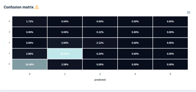
Example of Confusion Matrix for Multi-Class Classification in Provision.io
def accuracy(y_true, y_pred):
 """
 Function to calculate accuracy
 :param y_true: list of true values
 :param y_pred: list of predicted values
 :return: accuracy score
 """
 # initialize a simple counter for correct predictions
 correct_counter = 0
 # loop over all elements of y_true
 # and y_pred "together"
 for yt, yp in zip(y_true, y_pred):
 if yt == yp:
 # if prediction is equal to truth, increase the counter
 correct_counter += 1
 # return accuracy
 # which is correct predictions over the number of samples
 return correct_counter / len(y_true)
Error rate
Error rate is deduced from the previous Accuracy metric. In fact, Error rate = 1 – Accuracy.
def error_rate(y_true, y_pred):
 """
 Function to calculate accuracy
 :param y_true: list of true values
 :param y_pred: list of predicted values
 :return: accuracy score
 """
 # initialize a simple counter for correct predictions
 correct_counter = 0
 # loop over all elements of y_true
 # and y_pred "together"
 for yt, yp in zip(y_true, y_pred):
 if yt == yp:
 # if prediction is equal to truth, increase the counter
 correct_counter += 1
 # return accuracy
 # which is correct predictions over the number of samples
 return 1 - (correct_counter / len(y_true))
Multi Log Loss
Multi Log loss, aka logistic loss or cross-entropy loss measures the performance of a classification model whose output is a probability value between 0 and 1. Cross-entropy loss increases as the predicted probability diverges from the actual label. So predicting a probability of .012 when the actual observation label is 1 would be bad and result in a high loss value. A perfect model would have a log loss of 0.
In a multi-classification problem, we define the logarithmic loss function F in terms of the logarithmic loss function per label Fi as:
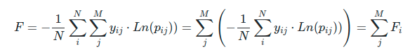
where :
- N is the number of instances,
- M is the number of different labels,
- yij is the binary variable with the expected labels
- pij is the classification probability output by the classifier for the i-instance and the j-label.
The cost function F measures the distance between two probability distributions, i.e. how similar is the distribution of actual labels and classifier probabilities. Hence, values close to zero are preferred.
import numpy as np
def log_loss(y_true, y_proba):
 """
 Function to calculate log loss
 :param y_true: list of true values
 :param y_proba: list of probabilities for 1
 :return: overall log loss
 """
 # define an epsilon value
 # this can also be an input
 # this value is used to clip probabilities
 epsilon = 1e-15
 # initialize empty list to store
 # individual losses
 loss = []
 # loop over all true and predicted probability values
 for yt, yp in zip(y_true, y_proba):
 # adjust probability
 # 0 gets converted to 1e-15
 # 1 gets converted to 1-1e-15
 # Why? Think about it!
 yp = np.clip(yp, epsilon, 1 - epsilon)
 # calculate loss for one sample
 temp_loss = - 1.0 * (
 yt * np.log(yp)
 + (1 - yt) * np.log(1 - yp)
 )
 # add to loss list
 loss.append(temp_loss)
 # return mean loss over all samples
 return np.mean(loss)
F1 Score
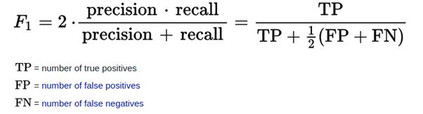
In statistical analysis of binary classification, the F-score or F-measure is a measure of a test’s accuracy. It is calculated from the precision and recall of the test, where the precision is the number of true positive results divided by the number of all positive results, including those not identified correctly, and the recall is the number of true positive results divided by the number of all samples that should have been identified as positive. Precision is also known as positive predictive value, and recall is also known as sensitivity in diagnostic binary classification.
The F1 score is the harmonic mean of precision and recall. The more generic {\displaystyle F_{\beta }}F_{\beta } score applies additional weights, valuing one of precision or recall more than the other.
The highest possible value of an F-score is 1.0, indicating perfect precision and recall, and the lowest possible value is 0, if either the precision or the recall is zero. [source]
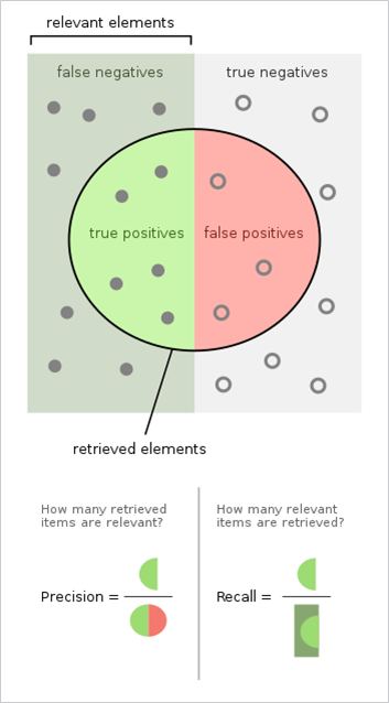
Precision / Recall définitions [source]
The F1 score can be interpreted as a weighted average of the precision and recall, where an F1 score reaches its best value at 1 and worst score at 0.
There are several versions of the F1 score depending on the expected granularity.
- micro: Calculate metrics globally by counting the total true positives, false negatives and false positives.
- macro: Calculate metrics for each label, and find their unweighted mean. This does not take label imbalance into account.
- weighted: Calculate metrics for each label, and find their average weighted by support (the number of true instances for each label). This alters ‘macro’ to account for label imbalance; it can result in an F-score that is not between precision and recall.
def true_positive(y_true, y_pred):
 """
 Function to calculate True Positives
 :param y_true: list of true values
 :param y_pred: list of predicted values
 :return: number of true positives
 """
 # initialize
 tp = 0
 for yt, yp in zip(y_true, y_pred):
 if yt == 1 and yp == 1:
 tp += 1
 return tp
def true_negative(y_true, y_pred):
 """
 Function to calculate True Negatives
 :param y_true: list of true values
 :param y_pred: list of predicted values
 :return: number of true negatives
 """
 # initialize
 tn = 0
 for yt, yp in zip(y_true, y_pred):
 if yt == 0 and yp == 0:
 tn += 1
 return tn
def false_positive(y_true, y_pred):
 """
 Function to calculate False Positives
 :param y_true: list of true values
 :param y_pred: list of predicted values
 :return: number of false positives
 """
 # initialize
 fp = 0
 for yt, yp in zip(y_true, y_pred):
 if yt == 0 and yp == 1:
 fp += 1
 return fp
def false_negative(y_true, y_pred):
 """
 Function to calculate False Negatives
 :param y_true: list of true values
 :param y_pred: list of predicted values
 :return: number of false negatives
 """
 # initialize
 fn = 0
 for yt, yp in zip(y_true, y_pred):
 if yt == 1 and yp == 0:
 fn += 1
 return fn

import numpy as np
def macro_precision(y_true, y_pred):
 """
 Function to calculate macro averaged precision
 :param y_true: list of true values
 :param y_pred: list of predicted values
 :return: macro precision score
 """

 # find the number of classes by taking
 # length of unique values in true list
 num_classes = len(np.unique(y_true))

 # initialize precision to 0
 precision = 0

 # loop over all classes
 for class_ in range(num_classes):

 # all classes except current are considered negative
 temp_true = [1 if p == class_ else 0 for p in y_true]
 temp_pred = [1 if p == class_ else 0 for p in y_pred]

 # calculate true positive for current class
 tp = true_positive(temp_true, temp_pred)

 # calculate false positive for current class
 fp = false_positive(temp_true, temp_pred)

 # calculate precision for current class
 temp_precision = tp / (tp + fp)

 # keep adding precision for all classes
 precision += temp_precision
 # calculate and return average precision over all classes
 precision /= num_classes
 return precision

import numpy as np
def micro_precision(y_true, y_pred):
 """
 Function to calculate micro averaged precision
 :param y_true: list of true values
 :param y_pred: list of predicted values
 :return: micro precision score
 """

 # find the number of classes by taking
 # length of unique values in true list
 num_classes = len(np.unique(y_true))

 # initialize tp and fp to 0
 tp = 0
 fp = 0

 # loop over all classes
 for class_ in range(num_classes):
 # all classes except current are considered negative
 temp_true = [1 if p == class_ else 0 for p in y_true]
 temp_pred = [1 if p == class_ else 0 for p in y_pred]

 # calculate true positive for current class
 # and update overall tp
 tp += true_positive(temp_true, temp_pred)

 # calculate false positive for current class
 # and update overall tp
 fp += false_positive(temp_true, temp_pred)

 # calculate and return overall precision
 precision = tp / (tp + fp)
 return precision


from collections import Counter
import numpy as np
def weighted_precision(y_true, y_pred):
 """
 Function to calculate weighted averaged precision
 :param y_true: list of true values
 :param y_pred: list of predicted values
 :return: weighted precision score
 """

 # find the number of classes by taking
 # length of unique values in true list
 num_classes = len(np.unique(y_true))

 # create class:sample count dictionary
 # it looks something like this:
 # {0: 20, 1:15, 2:21}
 class_counts = Counter(y_true)

 # initialize precision to 0
 precision = 0

 # loop over all classes
 for class_ in range(num_classes):
 # all classes except current are considered negative
 temp_true = [1 if p == class_ else 0 for p in y_true]
 temp_pred = [1 if p == class_ else 0 for p in y_pred]

 # calculate tp and fp for class
 tp = true_positive(temp_true, temp_pred)
 fp = false_positive(temp_true, temp_pred)

 # calculate precision of class
 temp_precision = tp / (tp + fp)

 # multiply precision with count of samples in class
 weighted_precision = class_counts[class_] * temp_precision

 # add to overall precision
 precision += weighted_precision
 # calculate overall precision by dividing by
 # total number of samples
 overall_precision = precision / len(y_true)
 return overall_precision
AUC
As we saw in the article Classification Metrics: [ADD LINK TO BINARY CLASSIFICATION POST], AUC (Area Under the ROC Curve), which measures the probability that a positive instance has a higher score than a negative instance, is a well-known performance metric for a scoring function’s ranking quality. AUC often comes up as a more appropriate performance metric than accuracy in various applications due to its appealing properties, e.g., insensitivity toward label distributions and costs. [source]
David J. Hand & Robert J. Till proposed in 2001 a simple generalization of the Area Under the ROC Curve for Multiple Class Classification Problems [source]
AUC values range from 0 to 1:
- AUC = 1 implies you have a perfect model. Most of the time, it means that
you made some mistake with validation and should revisit data processing
and holdout pipeline of yours. If you didn’t make any mistakes, then
congratulations, you have the best model one can have for the dataset you
built it on.
- AUC = 0 implies that your model is very bad (or very good!). Try inverting
the probabilities for the predictions, for example, if your probability for the
positive class is p, try substituting it with 1-p. This kind of AUC may also
mean that there is some problem with your validation or data processing.
- AUC = 0.5 implies that your predictions are random. So, for any binary
classification problem, if I predict all targets as 0.5, I will get an AUC of
0.5.
- AUC values between 0 and 0.5 imply that your model is worse than random. Most
of the time, it’s because you inverted the classes. If you try to invert your
predictions, your AUC might become more than 0.5. AUC values closer to 1 are
considered good.
from sklearn import metrics
metrics.roc_auc_score(y_true, y_pred)
Quadratic Weight Kappa (QWKP)
Quadratic Weight Kappa is also called Weighted Cohen’s Kappa.
Quadratic Weighted Kappa measures the agreement between two ratings. This metric typically varies from 0 (random agreement between raters) to 1 (complete agreement between raters). In the event that there is less agreement between the raters than expected by chance, the metric may go below 0. The quadratic weighted kappa is calculated between the scores which are expected/known and the predicted scores. [source]
Take the example of a multi class with N class. The quadratic weighted kappa is calculated as follows. First, an N x N histogram matrix O is constructed, such that Oi,j corresponds to the number of adoption records that have a rating of i (actual) and received a predicted rating j. An N-by-N matrix of weights, w, is calculated based on the difference between actual and predicted rating scores.
An N-by-N histogram matrix of expected ratings, E, is calculated, assuming that there is no correlation between rating scores. This is calculated as the outer product between the actual rating’s histogram vector of ratings and the predicted rating’s histogram vector of ratings, normalized such that E and O have the same sum.
From these three matrices, the quadratic weighted kappa is calculated.
- First, create a multi class confusion matrix O between predicted and actual ratings.
- Second, construct a weight matrix w which calculates the weight between the actual and predicted ratings.
- Third, calculate value_counts() for each rating in preds and actuals.
- Fourth, calculate E, which is the outer product of two value_count vectors
- Fifth, normalize the E and O matrix
Interpreting the Quadratic Weighted Kappa Metric
- A weighted Kappa is a metric which is used to calculate the amount of similarity between predictions and actuals. A perfect score of 1.0 is granted when both the predictions and actuals are the same.
- Whereas, the least possible score is -1 which is given when the predictions are furthest away from actuals.
- The aim is to get as close to 1 as possible. Generally a score of 0.6+ is considered to be a really good score.
from sklearn import metrics
metrics.cohen_kappa_score(y_true, y_pred, weights="quadratic")
service@provision.guru
The service@provision.guru metric measures the service@provision.guru for recommendations shown for different users and averages them over all queries in the dataset. The service@provision.guru metric is the most commonly used metric for evaluating recommender systems.
service@provision.guru all range from 0 to 1 with 1 being the best.
The mean average precision (mAP) of a set of queries is defined by Wikipedia as such:
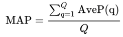
Mean average precision formula given provided by Wikipedia
where:
- Q is the number of queries in the set
- AveP(q) is the average precision (AP) for a given query q.
What the formula is essentially telling us is that, for a given query, q, we calculate its corresponding AP, and then the mean of all these AP scores would give us a single number, called the mAP, which quantifies how good our model is at performing the query.
def pk(y_true, y_pred, k):
 """
 This function calculates precision at k
 for a single sample
 :param y_true: list of values, actual classes
 :param y_pred: list of values, predicted classes
 :param k: the value for k
 :return: precision at a given value k
 """
 # if k is 0, return 0. we should never have this
 # as k is always >= 1
 if k == 0:
 return 0
 # we are interested only in top-k predictions
 y_pred = y_pred[:k]
 # convert predictions to set
 pred_set = set(y_pred)
 # convert actual values to set
 true_set = set(y_true)
 # find common values
 common_values = pred_set.intersection(true_set)
 # return length of common values over k
 return len(common_values) / len(y_pred[:k])

def apk(y_true, y_pred, k):
 """
 This function calculates average precision at k
 for a single sample
 :param y_true: list of values, actual classes
 :param y_pred: list of values, predicted classes
 :return: average precision at a given value k
 """
 # initialize service@provision.guru list of values
 pk_values = []
 # loop over all k. from 1 to k + 1
 for i in range(1, k + 1):
 # calculate service@provision.guru and append to list
 pk_values.append(pk(y_true, y_pred, i))
 # if we have no values in the list, return 0
 if len(pk_values) == 0:
 return 0
 # else, we return the sum of list over length of list
 return sum(pk_values) / len(pk_values)


def mapk(y_true, y_pred, k):
 """
 This function calculates mean avg precision at k
 for a single sample
 :param y_true: list of values, actual classes
 :param y_pred: list of values, predicted classes
 :return: mean avg precision at a given value k
 """
 # initialize empty list for apk values
 apk_values = []
 # loop over all samples
 for i in range(len(y_true)):
 # store apk values for every sample
 apk_values.append(
Approaching (Almost) Any Machine Learning Problem - Abhishek Thakur
64
 apk(y_true[i], y_pred[i], k=k)
 )
 # return mean of apk values list
 return sum(apk_values) / len(apk_values)
Multi Classifications metrics summary table
|
|
|
| Provision.io Notation |
| |||
Metric | Range | Lower is better | Weights accepted | 3 Stars | 2 Stars | 1 Star | 0 Star | Tips |
Multi LogLoss | 0 – ∞ | True | True | [0 ; 0.223[ | [0.223 ; 0.693[ | [0.693 ; +inf[ | – | Optimizes probabilities |
Macro F1 | 0 – 1 | False | True | ]0.85 ; 1] | ]0.65 ; 0.85] | ]0.5 ; 0.65] | [0 ; 0.5] | Equal weight on precision and recall |
Macro AUC | 0 – 1 | False | True | ]0.85 ; 1] | ]0.65 ; 0.85] | ]0.5 ; 0.65] | [0 ; 0.5] | Optimizes sort order of predictions |
Macro Accuracy | 0 – 1 | False | True | ]0.857 ; 1] | ]0.75 ; 0.857] | ]0.5 ; 0.75] | [0 ; 0.5] | Highly interpretable |
Quadratic Kappa | -1 – 1 | False | True | ]0.8 ; 1] | ]0.6 ; 0.8] | ]0.2 ; 0.6] | [-1 ; 0.2] |
|
0 – 1 | False | False | ]0.875 ; 1] | ]0.75 ; 0.875] | ]0.5 ; 0.75] | [0: 0.5] |
| |
Conclusion
We have introduced multi classification metrics, those implemented in Provision.io
In this article we have seen:
- the main multi classification metrics,
- their code implementation in Python,
- in which situations are they used,
- a summary table of these metrics.